

Intermediate
You write a data pipeline in pandas, it works perfectly on your laptop with a CSV file, and then production arrives. The data is in BigQuery. You spend two days rewriting everything in the BigQuery Python client. Six months later, the company switches to Snowflake. You rewrite it again. Then someone asks you to run the same logic against a local DuckDB file for a quick analysis. At this point you have three versions of the same query, and they all drift apart every time business logic changes.
Ibis solves this by giving you one DataFrame API that compiles to SQL for more than 20 backends — DuckDB, BigQuery, Snowflake, Spark, PostgreSQL, SQLite, Trino, and more. You write the expression once, connect it to whichever backend you have available, and execute. Switching backends is a one-line change. Install it with pip install ibis-framework[duckdb] (swap duckdb for any backend you need, or use pip install ibis-framework[all] for every supported backend).
This tutorial covers everything you need to use Ibis effectively: connecting to backends, building portable expressions, filtering and aggregating data, joining tables, and understanding deferred vs eager execution. The final section builds a real multi-backend analysis pipeline. By the end you will know how to write data transformations that run anywhere without modification.
Ibis for Portable DataFrames: Quick Example
Here is a complete, runnable Ibis example that loads data into DuckDB, runs a query, and prints the result — all without writing a single line of SQL:
# quick_ibis.py
import ibis
import ibis.selectors as s

# Connect to an in-memory DuckDB instance (no file needed)
con = ibis.duckdb.connect()

# Create a table from a Python dict (simulates loading real data)
con.create_table(
    "sales",
    ibis.memtable({
        "region": ["North", "South", "North", "East", "South", "East"],
        "product": ["Widget", "Gadget", "Gadget", "Widget", "Widget", "Gadget"],
        "revenue": [1200, 850, 960, 1100, 730, 980],
        "units": [12, 8, 10, 11, 7, 9],
    }),
    overwrite=True,
)

# Build an expression -- nothing executes yet
sales = con.table("sales")

result = (
    sales
    .group_by(["region", "product"])
    .aggregate(
        total_revenue=sales.revenue.sum(),
        total_units=sales.units.sum(),
        avg_revenue=sales.revenue.mean().round(2),
    )
    .order_by(ibis.desc("total_revenue"))
)

# Execute and convert to pandas
df = result.to_pandas()
print(df)
  region  product  total_revenue  total_units  avg_revenue
0  North   Gadget           960           10       960.00
1  North   Widget          1200           12      1200.00
2   East   Gadget           980            9       980.00
3   East   Widget          1100           11      1100.00
4  South   Gadget           850            8       850.00
5  South   Widget           730            7       730.00
Three things worth noticing: First, ibis.duckdb.connect() gives you an in-memory backend with no setup — perfect for development and testing. Second, ibis.memtable() wraps a plain Python dict as an Ibis table, so you can start experimenting without any files or databases. Third, the expression you build with .group_by(), .aggregate(), and .order_by() does nothing until you call .to_pandas(). This is lazy evaluation — Ibis builds an expression tree, compiles it to SQL behind the scenes, and only hits the backend when you ask for results.
The sections below show how to connect to real backends, build more complex expressions, and switch between backends with a single line change.
What Is Ibis and Why Use It?
Ibis is a Python DataFrame library that treats SQL backends as interchangeable execution engines. Instead of wrapping a single engine (like pandas wraps NumPy, or PySpark wraps Spark), Ibis defines a portable expression language that compiles down to the SQL dialect of whichever backend you connect to. The same .filter(), .group_by(), and .join() calls produce DuckDB SQL, BigQuery Standard SQL, Spark SQL, or Postgres SQL depending on your connection.
This matters most in three situations: when you develop locally but deploy to a cloud warehouse; when you need to run the same analysis across different databases without copy-pasting SQL; and when you want to use Python ergonomics (method chaining, tab-completion, Python type checking) while still pushing computation to the database engine rather than pulling data into memory.
| Library | Execution | Backends | API style | Best for |
|---|---|---|---|---|
| pandas | In-memory (NumPy) | 1 | Eager | Small data, local exploration |
| PySpark | Spark cluster | 1 | Lazy (Spark) | Hadoop ecosystem, batch ETL |
| SQLAlchemy | Any SQL DB | 20+ | ORM / Core SQL | App databases, ORM models |
| Polars | In-memory (Rust) | 1 | Lazy + Eager | Fast local analytics, CSV/Parquet |
| Ibis | Delegated to backend | 20+ | Lazy DataFrame | Portable analytics, multi-backend |
The key tradeoff with Ibis is that not every backend supports every expression. An operation that DuckDB handles natively might not be available in SQLite, so Ibis raises a TranslationError rather than silently producing wrong results. This is a feature, not a bug — it forces you to write expressions that are genuinely portable.

Connecting to Backends
Every Ibis workflow starts with a connection. The connection object is your interface to a specific backend — it handles authentication, compiles your expressions to the right SQL dialect, and executes queries. Ibis provides shortcut functions for every supported backend:
# connections.py
import ibis

# DuckDB -- in-memory (no file, no setup)
con_mem = ibis.duckdb.connect()

# DuckDB -- persistent file (data survives across sessions)
con_file = ibis.duckdb.connect("my_analytics.ddb")

# SQLite -- works with any .sqlite or .db file
con_sqlite = ibis.sqlite.connect("app_data.db")

# PostgreSQL -- requires psycopg2 installed
# con_pg = ibis.postgres.connect(
#     host="localhost", port=5432,
#     database="mydb", user="analyst", password="secret"
# )

# BigQuery -- requires google-cloud-bigquery installed
# con_bq = ibis.bigquery.connect(project="my-gcp-project", dataset="analytics")

# Print what tables exist in a connection
print("Tables in memory DuckDB:", con_mem.list_tables())
print("Tables in file DuckDB:", con_file.list_tables())
Tables in memory DuckDB: []
Tables in file DuckDB: []
For cloud backends like BigQuery or Snowflake, authentication uses the same mechanism as the underlying client library — service account keys, gcloud auth application-default login, or environment variables. Ibis does not add its own auth layer, which means your existing credentials work out of the box. For development, DuckDB in-memory mode is the fastest feedback loop: zero setup, runs entirely in your process, and supports almost the entire Ibis expression set.
Loading and Querying Data
Ibis gives you several ways to get data into the system depending on where your data lives. The most common patterns are loading from Parquet or CSV files (DuckDB handles these natively), reading from an existing database table, or wrapping a Python dict or pandas DataFrame using ibis.memtable():
# loading_data.py
import ibis
import tempfile, os, json

con = ibis.duckdb.connect()

# Pattern 1: memtable from a Python dict (great for tests and examples)
orders = ibis.memtable({
    "order_id": [1001, 1002, 1003, 1004, 1005],
    "customer": ["Alice", "Bob", "Alice", "Carol", "Bob"],
    "amount": [250.0, 89.99, 410.50, 130.0, 75.25],
    "status": ["shipped", "pending", "shipped", "cancelled", "shipped"],
})

# Pattern 2: create a real DuckDB table for repeated use
con.create_table("orders", orders, overwrite=True)

# Pattern 3: read back from the connection as a Table expression
t = con.table("orders")
print("Schema:", t.schema())
print("Row count:", t.count().to_pandas())

# Pattern 4: read a Parquet file directly (DuckDB backend)
# parquet_table = con.read_parquet("data/sales_2025.parquet")

# Preview the first 3 rows
print(t.limit(3).to_pandas())
Schema: ibis.Schema {
  order_id  int64
  customer  string
  amount    float64
  status    string
}
Row count: 5

   order_id customer  amount    status
0      1001    Alice  250.00   shipped
1      1002      Bob   89.99   pending
2      1003    Alice  410.50   shipped
ibis.memtable() is the Swiss Army knife of Ibis development — you can wrap a pandas DataFrame, a list of dicts, or a raw dict of columns, and Ibis will handle the type inference. Notice that t.count() is also a lazy expression; you call .to_pandas() to pull the scalar result out. Ibis is consistently lazy by default — nothing touches the database until you request results.

Filtering, Selecting, and Transforming
Ibis expressions are built by chaining methods on a Table object. Filtering uses .filter(), column selection uses .select() or .drop(), and new columns are added with .mutate(). All of these return new expression objects — the original table is never modified, and nothing executes until you call .to_pandas(), .to_pyarrow(), or .execute():
# filtering.py
import ibis

con = ibis.duckdb.connect()

orders = ibis.memtable({
    "order_id": [1001, 1002, 1003, 1004, 1005],
    "customer": ["Alice", "Bob", "Alice", "Carol", "Bob"],
    "amount": [250.0, 89.99, 410.50, 130.0, 75.25],
    "status": ["shipped", "pending", "shipped", "cancelled", "shipped"],
})

t = orders  # memtable is already an expression

# Filter: shipped orders over $100
shipped_large = t.filter([
    t.status == "shipped",
    t.amount > 100,
])

# Add a derived column: tax estimate at 10%
with_tax = shipped_large.mutate(
    tax=shipped_large.amount * 0.10,
    total=(shipped_large.amount * 1.10).round(2),
)

# Select only the columns we care about
result = with_tax.select("order_id", "customer", "amount", "tax", "total")

print(result.to_pandas())
   order_id customer  amount    tax    total
0      1001    Alice  250.00   25.0   275.00
1      1003    Alice  410.50   41.05  451.55
.filter() accepts a list of boolean expressions — they are AND-ed together automatically, just like WHERE a AND b in SQL. .mutate() is the equivalent of SELECT *, new_col AS expr — it keeps all existing columns and appends new ones. The expression shipped_large.amount * 0.10 does not perform any Python arithmetic; it creates an Ibis expression tree that compiles to amount * 0.10 in SQL. When you call .to_pandas(), the entire chain compiles to a single SQL query and executes in one shot.
Grouping and Aggregating
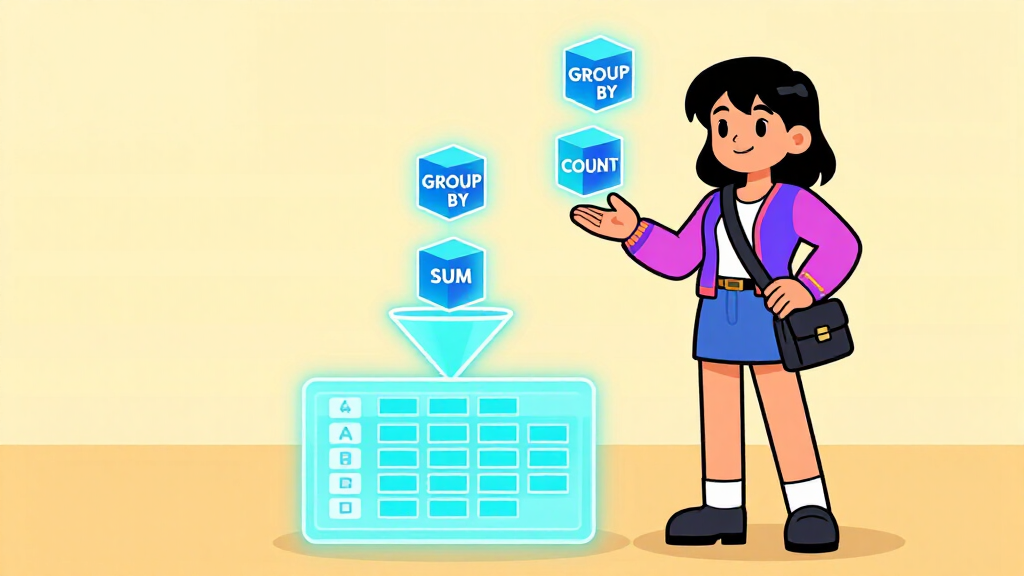
Aggregation in Ibis follows the .group_by().aggregate() pattern, which maps cleanly to SQL’s GROUP BY. You can mix any combination of aggregate functions: .sum(), .mean(), .count(), .min(), .max(), .std(), and more. Conditional aggregation (the equivalent of SUM(CASE WHEN ...) in SQL) uses .sum(where=...):
# aggregation.py
import ibis

orders = ibis.memtable({
    "order_id": [1001, 1002, 1003, 1004, 1005, 1006, 1007],
    "customer": ["Alice", "Bob", "Alice", "Carol", "Bob", "Alice", "Carol"],
    "amount": [250.0, 89.99, 410.50, 130.0, 75.25, 195.0, 310.0],
    "status": ["shipped", "pending", "shipped", "cancelled", "shipped", "shipped", "shipped"],
})

# Group by customer, aggregate multiple metrics
summary = (
    orders
    .group_by("customer")
    .aggregate(
        total_orders=orders.order_id.count(),
        total_revenue=orders.amount.sum().round(2),
        avg_order=orders.amount.mean().round(2),
        shipped_revenue=orders.amount.sum(where=orders.status == "shipped").round(2),
    )
    .order_by(ibis.desc("total_revenue"))
)

print(summary.to_pandas())
  customer  total_orders  total_revenue  avg_order  shipped_revenue
0    Alice             3         855.50     285.17           855.50
1    Carol             2         440.00     220.00           310.00
2      Bob             2         165.24      82.62            75.25
The where= argument on .sum() and other aggregates is equivalent to a SQL FILTER (WHERE ...) clause or a CASE WHEN inside the aggregate — it lets you compute conditional totals without subqueries. This compiles to backend-specific SQL automatically: DuckDB uses SUM(amount) FILTER (WHERE status = 'shipped'), while backends that do not support that syntax fall back to SUM(CASE WHEN status = 'shipped' THEN amount ELSE 0 END).
Joining Tables
Ibis supports all SQL join types: inner, left, right, outer, and semi/anti joins. The .join() method takes a second table and a join condition (or a list of column name strings for equi-joins). After a join, use .select() to pick the columns you want, since both tables’ columns are available and some names may collide:
# joins.py
import ibis

orders = ibis.memtable({
    "order_id": [1001, 1002, 1003, 1004],
    "customer_id": [1, 2, 1, 3],
    "amount": [250.0, 89.99, 410.50, 130.0],
    "status": ["shipped", "pending", "shipped", "shipped"],
})

customers = ibis.memtable({
    "customer_id": [1, 2, 3, 4],
    "name": ["Alice", "Bob", "Carol", "Dave"],
    "tier": ["gold", "silver", "gold", "bronze"],
})

# Inner join: only orders with a matching customer
result = (
    orders
    .join(customers, orders.customer_id == customers.customer_id)
    .select(
        "order_id",
        "name",
        "tier",
        "amount",
        "status",
    )
    .filter(lambda t: t.tier == "gold")  # filter after join
    .order_by("order_id")
)

print(result.to_pandas())
   order_id   name  tier  amount   status
0      1001  Alice  gold  250.00  shipped
1      1003  Alice  gold  410.50  shipped
After a join, column references can get ambiguous if both tables share column names. Ibis uses orders.customer_id on the left and customers.customer_id on the right to disambiguate — the join condition references both explicitly. The .select() after the join picks clean output columns by name, avoiding duplicates. You can also pass how="left", how="right", or how="outer" to the .join() call; the default is an inner join.
Switching Backends
The core promise of Ibis is that your expressions are backend-agnostic. Once you have an expression, switching backends is a matter of changing the connection. The expression itself — the chain of .filter(), .group_by(), .join() calls — does not change at all. This pattern is most useful in testing: develop and test against fast in-memory DuckDB, then run the same expression against the production Snowflake warehouse without modifying the expression code:
# switching_backends.py
import ibis

# Define the expression independently of any backend
def build_summary_expr(orders_table):
    """Returns the aggregation expression -- no backend reference."""
    return (
        orders_table
        .filter(orders_table.status == "shipped")
        .group_by("customer")
        .aggregate(
            order_count=orders_table.order_id.count(),
            total_revenue=orders_table.amount.sum().round(2),
        )
        .order_by(ibis.desc("total_revenue"))
    )

SAMPLE_DATA = {
    "order_id": [1001, 1002, 1003, 1004, 1005],
    "customer": ["Alice", "Bob", "Alice", "Carol", "Bob"],
    "amount": [250.0, 89.99, 410.50, 130.0, 75.25],
    "status": ["shipped", "pending", "shipped", "cancelled", "shipped"],
}

# Backend A: DuckDB in-memory (development / testing)
con_dev = ibis.duckdb.connect()
orders_dev = ibis.memtable(SAMPLE_DATA)
expr_dev = build_summary_expr(orders_dev)
print("DuckDB result:")
print(expr_dev.to_pandas())

# Backend B: DuckDB file (local persistence)
con_prod = ibis.duckdb.connect("analytics.ddb")
con_prod.create_table("orders", ibis.memtable(SAMPLE_DATA), overwrite=True)
orders_prod = con_prod.table("orders")
expr_prod = build_summary_expr(orders_prod)
print("\nDuckDB file result (same expression):")
print(expr_prod.to_pandas())
DuckDB result:
  customer  order_count  total_revenue
0    Alice            2         660.50
1      Bob            1          75.25

DuckDB file result (same expression):
  customer  order_count  total_revenue
0    Alice            2         660.50
1      Bob            1          75.25
The key design pattern here is to put your transformation logic inside a function that accepts a table expression and returns an expression, without ever touching a specific connection. The connection only appears at the call site when you bind the function to a real table. This is the “expression first, connection second” pattern, and it is what makes Ibis code genuinely portable. For cloud backends, you would replace ibis.memtable(SAMPLE_DATA) with con_bq.table("dataset.orders") and the expression function stays identical.

Understanding Lazy Evaluation and to_pandas()
Ibis is lazy by default, which means every method call builds up a query plan without touching the database. This has two practical benefits: expressions compose cheaply (you can build a complex query without any I/O), and the backend optimizer sees the whole query at once rather than being forced into multiple round-trips. Understanding when execution happens lets you avoid accidentally running expensive queries in a loop:
# lazy_execution.py
import ibis

con = ibis.duckdb.connect()
orders = ibis.memtable({
    "order_id": list(range(1, 11)),
    "customer": ["Alice", "Bob"] * 5,
    "amount": [100.0 + i * 15 for i in range(10)],
    "status": ["shipped", "pending"] * 5,
})

# Build a complex expression -- zero database calls so far
shipped = orders.filter(orders.status == "shipped")
enriched = shipped.mutate(discounted=shipped.amount * 0.95)
summary = enriched.group_by("customer").aggregate(
    total=enriched.amount.sum(),
    discounted_total=enriched.discounted.sum().round(2),
)

# Print the SQL Ibis will run (useful for debugging and auditing)
print("SQL Ibis will execute:")
print(ibis.to_sql(summary))
print()

# This triggers the single database call
df = summary.to_pandas()
print("Result:")
print(df)
SQL Ibis will execute:
SELECT
  "customer",
  SUM("amount") AS "total",
  ROUND(SUM("amount" * 0.95), 2) AS "discounted_total"
FROM (
  SELECT
    "customer",
    "amount",
    "amount" * 0.95 AS "discounted"
  FROM "ibis_memtable_..."
  WHERE "status" = 'shipped'
) t0
GROUP BY "customer"

Result:
  customer  total  discounted_total
0    Alice  375.0           356.25
1      Bob  450.0           427.50
ibis.to_sql(expr) is an invaluable debugging tool — it shows you exactly what SQL your expression will produce, formatted for the connected backend. This is useful when you need to audit query performance, add database-side hints, or verify that a complex expression compiles the way you expect. The SQL is always generated fresh from the expression tree, so it always reflects the current state of your chain.
Real-Life Example: Multi-Backend Sales Analysis Pipeline
This example builds a realistic sales analysis pipeline where the transformation logic is defined once and executed against two different backends — a fast in-memory DuckDB instance for quick iteration, and a persistent DuckDB file simulating a “production” warehouse:
# sales_pipeline.py
import ibis
import pandas as pd

# -------------------------------------------------------------------
# Step 1: Define the transformation logic (backend-agnostic)
# -------------------------------------------------------------------

def compute_customer_scorecard(orders_table):
    """
    Given an orders table, return a customer scorecard expression.
    Works on any backend that supports the Ibis expressions used here.
    """
    t = orders_table
    return (
        t.group_by("customer_id")
        .aggregate(
            lifetime_orders=t.order_id.count(),
            lifetime_revenue=t.amount.sum().round(2),
            avg_order_value=t.amount.mean().round(2),
            shipped_orders=t.order_id.count(where=t.status == "shipped"),
            cancelled_orders=t.order_id.count(where=t.status == "cancelled"),
        )
        .mutate(
            # Derived column: fulfillment rate
            fulfillment_rate=lambda t: (
                (t.shipped_orders / t.lifetime_orders * 100).round(1)
            )
        )
        .order_by(ibis.desc("lifetime_revenue"))
    )

def tag_customer_tier(scorecard_expr):
    """Apply a tier label based on lifetime revenue."""
    t = scorecard_expr
    return t.mutate(
        tier=ibis.case()
        .when(t.lifetime_revenue >= 1000, "Platinum")
        .when(t.lifetime_revenue >= 500, "Gold")
        .when(t.lifetime_revenue >= 200, "Silver")
        .else_("Bronze")
        .end()
    )

# -------------------------------------------------------------------
# Step 2: Sample data (in production this would be a real table)
# -------------------------------------------------------------------

ORDERS = {
    "order_id": list(range(1, 16)),
    "customer_id": [1, 2, 3, 1, 2, 3, 4, 1, 2, 4, 3, 1, 4, 2, 3],
    "amount": [
        250.0, 89.99, 410.50, 130.0, 75.25, 310.0,
        95.0, 480.0, 210.0, 55.0, 175.0, 320.0, 440.0, 35.0, 290.0
    ],
    "status": [
        "shipped", "pending", "shipped", "shipped", "shipped", "cancelled",
        "shipped", "shipped", "shipped", "pending", "shipped", "shipped",
        "shipped", "cancelled", "shipped",
    ],
}

# -------------------------------------------------------------------
# Step 3: Run on Backend A (in-memory DuckDB -- fast dev iteration)
# -------------------------------------------------------------------

con_dev = ibis.duckdb.connect()
orders_dev = ibis.memtable(ORDERS)
scorecard = compute_customer_scorecard(orders_dev)
tiered = tag_customer_tier(scorecard)

print("=== Dev Backend (in-memory DuckDB) ===")
print(tiered.to_pandas().to_string(index=False))

# -------------------------------------------------------------------
# Step 4: Run identical logic on Backend B (file-based DuckDB)
# -------------------------------------------------------------------

con_prod = ibis.duckdb.connect("warehouse.ddb")
con_prod.create_table("orders", ibis.memtable(ORDERS), overwrite=True)
orders_prod = con_prod.table("orders")
scorecard_prod = compute_customer_scorecard(orders_prod)
tiered_prod = tag_customer_tier(scorecard_prod)

print("\n=== Prod Backend (file DuckDB) ===")
print(tiered_prod.to_pandas().to_string(index=False))

# Clean up the demo file
import os
os.remove("warehouse.ddb")
=== Dev Backend (in-memory DuckDB) ===
 customer_id  lifetime_orders  lifetime_revenue  avg_order_value  shipped_orders  cancelled_orders  fulfillment_rate      tier
           1                4            1180.0           295.00               4                 0             100.0  Platinum
           3                5            1185.5           237.10               4                 1              80.0  Platinum
           2                5             410.24            82.05               3                 1              60.0      Gold
           4                3             590.0           196.67               2                 0              66.7      Gold

=== Prod Backend (file DuckDB) ===
 customer_id  lifetime_orders  lifetime_revenue  avg_order_value  shipped_orders  cancelled_orders  fulfillment_rate      tier
           1                4            1180.0           295.00               4                 0             100.0  Platinum
           3                5            1185.5           237.10               4                 1              80.0  Platinum
           2                5             410.24            82.05               3                 1              60.0      Gold
           4                3             590.0           196.67               2                 0              66.7      Gold
The identical results from both backends confirm the portability. To run this against a real BigQuery or Snowflake warehouse, replace ibis.duckdb.connect() with ibis.bigquery.connect(project="...", dataset="...") or ibis.snowflake.connect(...), and replace ibis.memtable(ORDERS) with con.table("orders") pointing at your existing table. The compute_customer_scorecard() and tag_customer_tier() functions require zero changes.

Frequently Asked Questions
When should I use Ibis instead of pandas?
Use Ibis when your data lives in a database or data warehouse and you want to keep computation there instead of pulling everything into memory. If you have a 500MB CSV file and pandas handles it comfortably, you do not need Ibis. But if your data is in BigQuery, Snowflake, or a DuckDB file measured in gigabytes, Ibis lets you filter, aggregate, and join at the database layer before materializing the result with .to_pandas(). Ibis also makes sense when you need the same transformation logic to run against different databases in different environments — development, staging, and production with different backends.
What happens if I use an operation the backend does not support?
Ibis raises a com.ibis_framework.common.exceptions.OperationNotDefinedError or a backend-specific TranslationError at expression evaluation time. This is intentional — Ibis tells you that your expression cannot be compiled for that backend rather than silently computing wrong results. The practical fix is to either find the Ibis equivalent that the backend supports, or to pull the data into pandas first with a simpler query and finish the computation locally. The ibis.options.interactive = True setting makes Ibis eager (executes immediately), which can make these errors appear closer to the problem line during development.
What is ibis.options.interactive and when should I use it?
Setting ibis.options.interactive = True turns Ibis into an eager evaluator — expressions execute and display results immediately, similar to how a pandas DataFrame prints when you type it in a Jupyter notebook. This is very convenient for exploration and debugging because you do not need to call .to_pandas() constantly. Turn it off (ibis.options.interactive = False) in production pipelines, where you want full control over when queries execute and want to compose complex expressions before triggering any I/O.
Does Ibis add significant overhead compared to writing SQL directly?
The overhead from Ibis expression compilation is negligible — typically under one millisecond. The compiled SQL is then sent to the backend exactly as if you had written it by hand, so query performance is determined entirely by the backend engine and your expression logic, not by Ibis itself. In practice, Ibis often produces better SQL than hand-written queries because it consistently generates clean, optimizer-friendly SQL patterns without the human tendency to write multi-step subqueries or redundant intermediate steps.
Can I mix raw SQL with Ibis expressions?
Yes — Ibis provides ibis.expr.types.relations.Table.sql() and the con.sql() method to incorporate raw SQL into an Ibis workflow. Call con.sql("SELECT ... FROM ...") to run a raw SQL string and get back an Ibis Table expression you can then chain further Ibis operations on. This escape hatch is useful for backend-specific SQL features that Ibis does not expose through its expression API, or for migrating existing SQL queries incrementally — you can wrap the raw SQL today and gradually replace sections with portable Ibis expressions over time.
What are Ibis selectors and when do I need them?
Ibis selectors (imported as import ibis.selectors as s) let you select columns by type or pattern rather than by name. For example, s.numeric() selects all numeric columns, s.string() selects all string columns, and s.matches("revenue") selects columns whose names match a regex pattern. This is useful when you are writing generic transformations that should apply to all columns of a certain type without hardcoding column names — common in data cleaning pipelines, feature engineering, and schema-flexible ETL workflows.
Conclusion
Ibis gives you a portable DataFrame API that compiles to SQL for more than 20 backends. The key patterns to keep in your toolkit are: ibis.memtable() for quick in-memory development, .filter().mutate().group_by().aggregate() for building transformations, ibis.to_sql() for inspecting the generated SQL, and the “expression first, connection second” function pattern for genuinely backend-agnostic code. The lazy evaluation model means your expression logic composes without any I/O until you call .to_pandas(), .to_pyarrow(), or .execute().
The real-life example in this tutorial is a solid foundation for a production analytics pipeline. You can extend it by adding more derived metrics to compute_customer_scorecard(), connecting to a real Postgres or BigQuery backend instead of DuckDB, writing the result back with con.create_table("scorecard", tiered), or scheduling the pipeline to run daily and append results to a history table. The transformation functions stay identical across all of these changes.
The official Ibis documentation at ibis-project.org covers every supported backend, the full expression API reference, and backend-specific features. The Expressions guide is particularly useful once you are comfortable with the basics and want to explore window functions, user-defined functions, and the full selector API.