
Last Updated: June 01, 2026
Advanced
Making computer generated text mimic human speech is fascinating and actually not that difficult for an effect that is sometimes convincing, but certainly entertaining. Markov Chain’s is one way to do this. It works by generating new text based on historical texts where the original sequencing of neighboring words (or groups of words) is used to generate meaningful sentences. Read the below guide on how to code a Markov Chain text generator (code example in python) including explanation of the concept.
What’s really interesting, is that you can take historical texts of a person, then generate new sentences which can sound similar to the way that person speaks. Alternatively, you can combine texts from two different people and get a mixed “voice”.
I played around this with texts of speeches from two great presidents:

What my Markov Chain generated which was “trained” using the combination of texts from Obama speeches and Bartlet scripts, is as follows:
- ‘Can I burn my mother in North Carolina for giving us a great night planned.’
- ‘And so going forward, I believe that we can build a bomb into their church.’
- ‘’Charlie, my father had grown up in the Situation Room every time I came in.’’
- ‘This campaign must be ballistic.’,

Python developer and educator with 15+ years building production systems across data engineering, web APIs, and AI tooling. Founder of Python How To Program — 270+ in-depth tutorials covering the modern Python stack.
What is a Markov Chain in the context of a text generation?
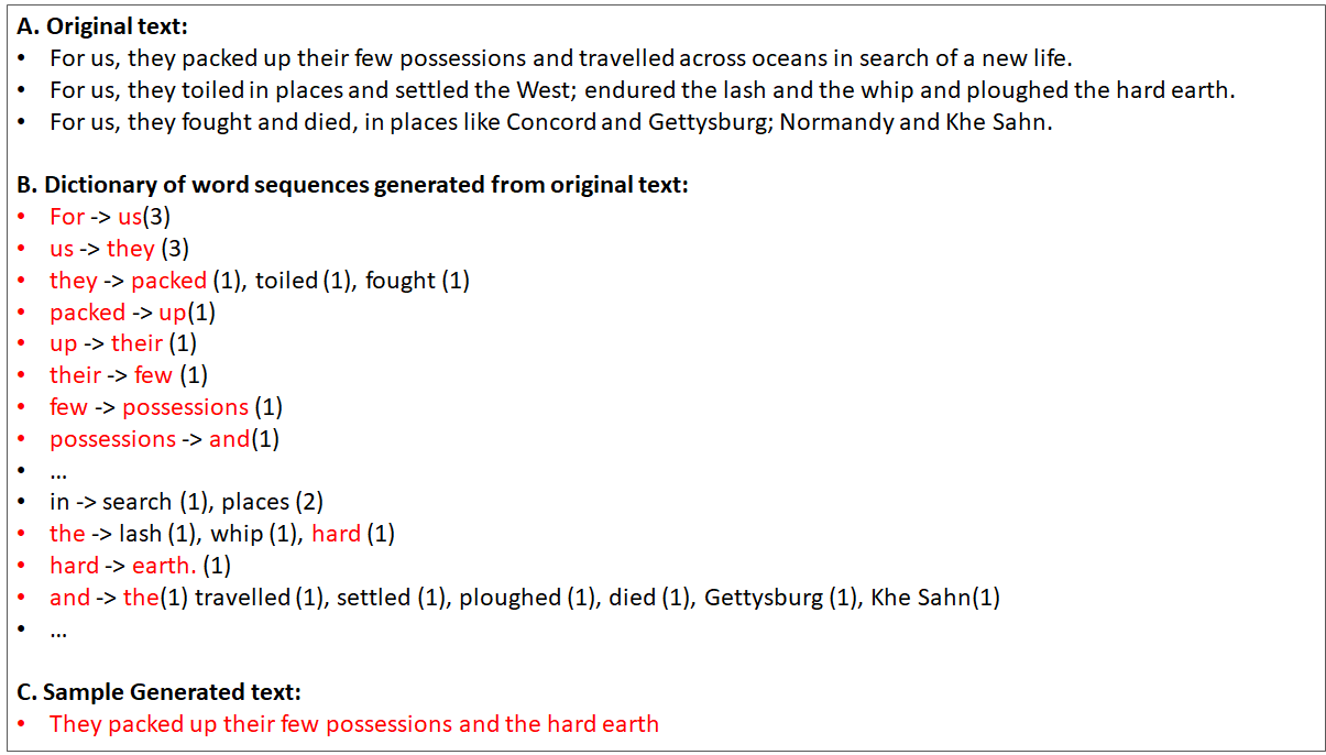
For a more technical explanation, I think you can find plenty of resources out there. In simple terms, it is an algorithm which is used to generate a new outcome from a weighted list of words based on historical texts. Now that’s rather abstract. In more practical terms, in the scenario for text generation, it is a way to use historical texts, chop it up into individual words (or sets of words), and then randomly chose a given word then randomly chose the next likely words based on historical sequences. For example:
This doesn’t just apply in text as well (although one of the most popular applications is in your smart phone where there’s predictive text), it can be used for any scenario where you use historical information to define next steps for a given state. For example, you could codify a given stock market pattern (such as the % daily changes for the last 30 days), then use that to see historically what was the likely next day outcome (example only.. I’m very doubtful how effective it would be).
Why are Markov Chain Text Generators so fun?
I’ve always wanted to build a text generator as it’s just an awesome way to see how you could mimic intelligence using a very cheap shortcut. You’ll see the algorithm below, and it is super simple. The other fact is that, like above example, you can use it to mix the ‘voice’ from two different persons and see the outcome.
How does the Markov Chain Text Generator work?
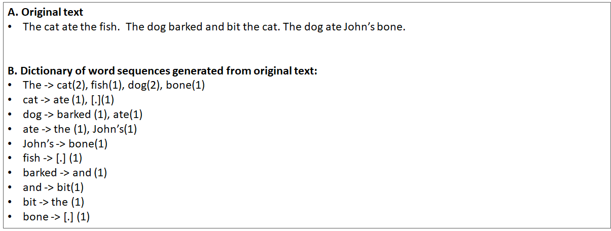
There are two phases for text generation with Markov Chains. There’s first the ‘dictionary build phase’ which involves gathering the historical texts, and then generating a dictionary with the key being a given word in a sentence, and then having the resultant being the natural follow-up words.
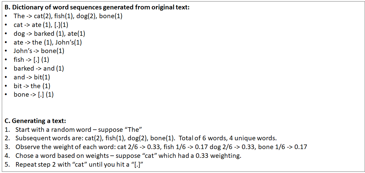
The second is the execution, where you start from a given word, then use that word to see what the next word would be in a probabilistic way. For example:
Now, there are some tricks which you need to be mindful of ( I found this out the hard way):
- You can’t start from any random word — if you do, then you’ll get sentences like this: “ate the cat.” . You have to keep track of “starting words” to keep things simple — hence you can have: “John ate the cat”.
- Don’t ignore punctuation— if you do remove punctuation, you’ll get sentence like this: “The dog barked at John cat”. Instead keep them there so that you can have a better chance to have a more realistic sentence — i.e. “The dog barked at John’s ca”
- End on a full-stop word. When you go through and start from a word, then find the next word, then find the next word and so on, you can continue until you reach a specified length, but then you’ll end up stopping in mid-sentence such as this: “The cat ate John’s”. Instead, simply end when you have a word that has a full stop (another reason not to remove the punctuation) — i.e. “The cat ate John’s boots.”
Markov Chain Example Code Source texts
I played around with different texts including: Eddie Murphy stand-up routines, Donald Trump tweets, Obama speeches, and Jed Bartlet dialogue. You can find the the markov chain example source text here. It’s great to use one source and then generate the dictionary, but then you can mix and match and use two sources (e.g. Obama and Bartlet) and then create the one dictionary file. Then when you traverse the dictionary you get the both voices.
It is important to make sure that you can balance the text — e.g. if you had a 8000 text from Obama and only 1000 text from Eddie Murphy, it’s likely that you would see more of the Obama words. Of course, when you build the dictionary, you can also add some artificial weighting towards the lighter text source to balance things out.
Markov Chain Summary
The Markov Chain text generator is not perfect — you’ll see when you create your own, that some text is just gibberish. The more text that you have the better. Secondly, using single words is not helpful in the dictionary — you should use groups of 2–3 words. The actual number depends on how much historical text you have.
You can find all the python code, source texts and Markov Chain python example code here. Good luck!
Subscribe to our newsletter

How To Use PyArrow for Parquet File Processing in Python
Intermediate
You have a CSV file with ten million rows of sales data. You read it into pandas every morning, filter down to the last 30 days, and compute some aggregates. The read step alone takes 45 seconds. Now imagine it took less than two. That is the promise of Parquet — a columnar binary file format designed for exactly this kind of workload. Instead of reading every row to find the values in a single column, Parquet lets the engine skip straight to the data it actually needs.
PyArrow is the Python library that makes Parquet accessible without any special infrastructure. It ships with pandas, integrates with polars, and lets you read and write Parquet files in a handful of lines of code. PyArrow also handles schema enforcement, Snappy and Zstandard compression, and partitioned datasets spread across directories — the same building blocks that power data lakes at companies like Uber and Netflix, available on your laptop.
In this article we will cover how to install PyArrow and write your first Parquet file, how the columnar format differs from CSV and JSON, how to control schema and compression, how to filter data at read time without loading the whole file, how to work with partitioned Parquet datasets, and how to build a real-world pipeline that stores transaction data efficiently. By the end you will have a working toolkit for replacing slow CSV pipelines with fast, schema-safe Parquet files.
PyArrow Parquet in Python: Quick Example
Here is a self-contained example that creates a table, writes it to Parquet, reads it back, and prints the result — all in about 15 lines:
# quick_parquet.py
import pyarrow as pa
import pyarrow.parquet as pq

# Create an Arrow table from Python lists
table = pa.table({
    "product": ["Widget A", "Widget B", "Widget C"],
    "quantity": [100, 250, 75],
    "price": [9.99, 4.49, 19.99],
})

# Write to Parquet
pq.write_table(table, "products.parquet")

# Read it back
result = pq.read_table("products.parquet")
print(result.to_pandas())
Output:
    product  quantity  price
0  Widget A       100   9.99
1  Widget B       250   4.49
2  Widget C        75  19.99
The two key functions are pq.write_table() and pq.read_table(). Both take a file path as their second argument. pa.table() creates an Arrow table from a dictionary of column names to Python lists — PyArrow infers the data types automatically. You get a typed, compressed binary file on disk and a clean DataFrame-compatible object back on read.
That is the core loop. The rest of this article shows you how to control compression, enforce schemas, filter at read time, and partition data across directories for datasets that do not fit in memory.

What Is Parquet and Why Is It Faster Than CSV?
Parquet is a columnar storage format originally developed at Twitter and Cloudera for the Hadoop ecosystem. Instead of storing data row by row (like CSV or JSON), Parquet stores all the values in each column together. This has three major consequences: better compression, faster column scans, and cheaper predicate pushdown.
When values in the same column are stored together, they tend to be similar in type and often in value — a “country” column full of repeated strings like “AU” or “US” compresses dramatically compared to mixed-content rows. A Parquet file is also self-describing: it embeds a schema with column names and types, so you never have to guess whether a field is a string or a number.
Here is how the main file formats compare for typical data engineering workloads:
| Feature | CSV | JSON | Parquet |
|---|---|---|---|
| Storage format | Row-oriented text | Row-oriented text | Column-oriented binary |
| Schema embedded | No | No | Yes |
| Compression | None (plain text) | None | Snappy, Gzip, Zstd |
| Read a single column | Must scan entire file | Must scan entire file | Jumps directly to column |
| Predicate pushdown | Not supported | Not supported | Row group filtering |
| Typical file size | Large | Larger | 3x-10x smaller |
| Human readable | Yes | Yes | No (binary) |
The tradeoff is binary format — you cannot open a Parquet file in a text editor. But for data pipelines that read the same file repeatedly, the speed and size advantages far outweigh the loss of human readability. PyArrow bridges this gap by making the format as easy to work with as CSV.
Writing Parquet Files with PyArrow
You can create Parquet files from PyArrow tables, pandas DataFrames, or plain Python dictionaries. The most direct path is pa.table() followed by pq.write_table(). PyArrow automatically infers the schema from your data types unless you supply one explicitly.
# write_parquet.py
import pyarrow as pa
import pyarrow.parquet as pq
import pandas as pd

# Method 1: from a pandas DataFrame
df = pd.DataFrame({
    "user_id": [1001, 1002, 1003, 1004],
    "country": ["AU", "US", "AU", "GB"],
    "spend": [120.50, 88.00, 200.75, 44.20],
    "active": [True, False, True, True],
})
table = pa.Table.from_pandas(df)
pq.write_table(table, "users.parquet")

# Method 2: directly from an Arrow table
orders = pa.table({
    "order_id": pa.array([5001, 5002, 5003], type=pa.int32()),
    "amount": pa.array([29.99, 14.50, 99.00], type=pa.float64()),
    "status": pa.array(["shipped", "pending", "delivered"], type=pa.string()),
})
pq.write_table(orders, "orders.parquet", compression="snappy")
print("Files written.")
Output:
Files written.
Notice compression="snappy" in the second call. Snappy is the default when compression is not specified — it is fast to decode and gives reasonable size reduction. You can also use "gzip" for better compression at the cost of slower reads, or "zstd" for the best balance of speed and compression ratio. For data you read frequently, Snappy is usually the right choice. For archival data you read rarely, Zstd at a higher compression level saves more disk space.
Reading Parquet Files and Filtering Columns
Reading a full Parquet file is one line. The real power comes from reading only the columns you need — PyArrow loads only those column chunks from disk, skipping the rest entirely. For a 100-column dataset where your query uses only 3 columns, this can be a 30x reduction in I/O.
# read_parquet.py
import pyarrow.parquet as pq

# Read all columns
full = pq.read_table("users.parquet")
print("Full table:")
print(full.to_pandas())
print()

# Read only specific columns -- PyArrow skips the others on disk
subset = pq.read_table("users.parquet", columns=["user_id", "country"])
print("Subset (2 of 4 columns):")
print(subset.to_pandas())
Output:
Full table:
   user_id country   spend  active
0     1001      AU  120.50    True
1     1002      US   88.00   False
2     1003      AU  200.75    True
3     1004      GB   44.20    True

Subset (2 of 4 columns):
   user_id country
0     1001      AU
1     1002      US
2     1003      AU
3     1004      GB
PyArrow also supports predicate pushdown via the filters parameter. You can push filter conditions into the read operation so that row groups that cannot satisfy the filter are skipped without being decoded. For large files split into many row groups, this can cut read time dramatically.
# read_filtered.py
import pyarrow.parquet as pq

# Only return rows where country == "AU"
# Parquet row group statistics let PyArrow skip non-matching groups
au_users = pq.read_table(
    "users.parquet",
    filters=[("country", "==", "AU")],
)
print(au_users.to_pandas())
Output:
   user_id country   spend  active
0     1001      AU  120.50    True
1     1003      AU  200.75    True
The filters parameter accepts a list of tuples in the form (column, operator, value). Valid operators include ==, !=, <, >, <=, >=, in, and not in. For maximum effectiveness, sort your data by the filter column before writing — that way each row group contains a contiguous range and PyArrow can skip most groups on a range filter.

Defining and Enforcing Schemas
One of Parquet’s greatest strengths over CSV is explicit schema. When you read a CSV with mixed data, you often get silent type coercions — a column that should be integers becomes floats because one row had a decimal. With Parquet, the schema is embedded in the file and enforced on write. You can also define the schema explicitly and have PyArrow reject data that does not conform.
# schema_parquet.py
import pyarrow as pa
import pyarrow.parquet as pq

# Define an explicit schema with precise types
schema = pa.schema([
    pa.field("transaction_id", pa.int64()),
    pa.field("amount", pa.float64()),
    pa.field("currency", pa.string()),
    pa.field("timestamp", pa.timestamp("ms")),
])

# Create table with matching data
import pandas as pd
from datetime import datetime

df = pd.DataFrame({
    "transaction_id": [9001, 9002, 9003],
    "amount": [150.00, 32.50, 899.99],
    "currency": ["AUD", "USD", "EUR"],
    "timestamp": [
        datetime(2026, 6, 1, 9, 0),
        datetime(2026, 6, 1, 10, 15),
        datetime(2026, 6, 1, 11, 30),
    ],
})

# Cast to explicit schema -- raises if types are incompatible
table = pa.Table.from_pandas(df, schema=schema)
pq.write_table(table, "transactions.parquet")

# Read back and inspect schema
t = pq.read_table("transactions.parquet")
print(t.schema)
Output:
transaction_id: int64
amount: double
currency: string
timestamp: timestamp[ms]
The pa.schema() call creates a strict type contract for the file. If you try to write a DataFrame where transaction_id is a string, PyArrow raises a ArrowInvalid error at write time — not a silent runtime bug hours later. The pa.timestamp("ms") type stores timestamps as milliseconds since Unix epoch, which Parquet encodes compactly and PyArrow converts back to Python datetime objects automatically on read.
Choosing the Right Compression
Parquet supports several compression codecs. Each has different tradeoffs between file size and read/write speed. The right choice depends on your access pattern: if you write once and read many times (analytical workloads), optimize for read speed. If you archive data rarely accessed, optimize for size.
# compression_comparison.py
import pyarrow as pa
import pyarrow.parquet as pq
import os

table = pa.table({
    "category": ["electronics"] * 50000 + ["clothing"] * 50000,
    "value": list(range(100000)),
    "note": ["sample data for compression test"] * 100000,
})

codecs = ["none", "snappy", "gzip", "zstd"]

for codec in codecs:
    fname = f"data_{codec}.parquet"
    pq.write_table(table, fname, compression=codec)
    size_kb = os.path.getsize(fname) / 1024
    print(f"{codec:8s} -> {size_kb:8.1f} KB")
Output:
none     ->   2841.2 KB
snappy   ->    312.4 KB
gzip     ->    204.8 KB
zstd     ->    189.3 KB
Snappy achieves a 9x size reduction over uncompressed and is fast enough that decompression overhead is barely noticeable. Gzip and Zstd go further — typically 12x to 15x smaller — but take slightly longer to read. For most production pipelines, snappy is the default for a good reason. Switch to zstd (with compression_level=3) for cold archival storage where read latency matters less.

Working with Partitioned Datasets
When a dataset grows beyond what fits in a single file, you can partition it — split it across multiple Parquet files organized in a directory hierarchy. Hive-style partitioning uses subdirectory names like country=AU/ or year=2026/month=06/ to encode partition values. PyArrow reads partitioned datasets as if they were a single table, pushing partition filters at the directory level so entire directories are skipped without opening any files.
# partitioned_write.py
import pyarrow as pa
import pyarrow.dataset as ds
import pyarrow.parquet as pq
import shutil, os

table = pa.table({
    "user_id": [1, 2, 3, 4, 5, 6],
    "country": ["AU", "US", "AU", "GB", "US", "AU"],
    "spend": [120.5, 88.0, 200.75, 44.2, 310.0, 55.0],
})

output_dir = "partitioned_users"
if os.path.exists(output_dir):
    shutil.rmtree(output_dir)

# Write partitioned by country -- creates subdirs like country=AU/
pq.write_to_dataset(table, root_path=output_dir, partition_cols=["country"])

# Show what was created
for root, dirs, files in os.walk(output_dir):
    for f in files:
        path = os.path.join(root, f)
        print(path)
Output:
partitioned_users/country=AU/part-0.parquet
partitioned_users/country=GB/part-0.parquet
partitioned_users/country=US/part-0.parquet
Reading the partitioned dataset back is equally simple. PyArrow discovers all the partition directories and reconstructs the full table. You can also filter at the partition level — when you filter on country == "AU", PyArrow only opens the country=AU/ directory and never touches the others.
# partitioned_read.py
import pyarrow.dataset as ds

# Read only AU records -- other country dirs are skipped entirely
dataset = ds.dataset("partitioned_users", format="parquet", partitioning="hive")
au_data = dataset.to_table(filter=ds.field("country") == "AU")
print(au_data.to_pandas())
Output:
   user_id country   spend
0        1      AU  120.50
1        3      AU  200.75
2        6      AU   55.00
The partitioning="hive" argument tells PyArrow to expect Hive-style directory names. The ds.field("country") == "AU" expression is evaluated at the directory level — PyArrow reads the directory listing, sees that only country=AU/ matches, and skips country=US/ and country=GB/ completely.

PyArrow and pandas: Interoperability
If you already use pandas, PyArrow integrates cleanly in both directions. pandas.read_parquet() and pandas.DataFrame.to_parquet() use PyArrow under the hood when PyArrow is installed. You can pass PyArrow-specific options through pandas using the engine="pyarrow" argument.
# pandas_parquet.py
import pandas as pd

# Write from pandas
df = pd.DataFrame({
    "product_id": [101, 102, 103],
    "name": ["Bolt M6", "Nut M6", "Washer M6"],
    "stock": [500, 1200, 800],
    "unit_price": [0.10, 0.05, 0.03],
})
df.to_parquet("products_pd.parquet", engine="pyarrow", compression="snappy", index=False)

# Read from pandas -- column pruning still works
df_back = pd.read_parquet(
    "products_pd.parquet",
    engine="pyarrow",
    columns=["product_id", "name", "stock"],
)
print(df_back)
print(df_back.dtypes)
Output:
   product_id       name  stock
0         101    Bolt M6    500
1         102     Nut M6   1200
2         103  Washer M6    800
product_id      int64
name           object
stock           int64
dtype: object
Note index=False in the to_parquet() call. By default, pandas writes the DataFrame index as an extra column. For most datasets the index is just a sequential integer you do not need, so index=False keeps the file clean. If you are using a meaningful index (like timestamps), omit that argument and PyArrow will preserve it.
Real-Life Example: Daily Sales Archive Pipeline
Here is a realistic pipeline that reads daily sales data from CSV, validates the schema, writes partitioned Parquet files by date, and reads back aggregate statistics — the kind of pattern you would use to replace a slow nightly ETL job.
# sales_pipeline.py
import pyarrow as pa
import pyarrow.parquet as pq
import pyarrow.dataset as ds
import pandas as pd
import io, os, shutil

# --- Simulate raw CSV data arriving daily ---
raw_csv = """order_id,date,region,product,quantity,revenue
1001,2026-06-01,AU,Widget A,10,99.90
1002,2026-06-01,US,Widget B,5,22.45
1003,2026-06-02,AU,Widget A,3,29.97
1004,2026-06-02,GB,Widget C,8,159.92
1005,2026-06-03,US,Widget A,12,119.88
1006,2026-06-03,AU,Widget C,2,39.98
"""

# --- Step 1: Load and validate schema ---
schema = pa.schema([
    pa.field("order_id", pa.int64()),
    pa.field("date", pa.string()),
    pa.field("region", pa.string()),
    pa.field("product", pa.string()),
    pa.field("quantity", pa.int32()),
    pa.field("revenue", pa.float64()),
])

df = pd.read_csv(io.StringIO(raw_csv))
table = pa.Table.from_pandas(df, schema=schema)
print(f"Loaded {len(table)} rows with schema:")
print(table.schema)

# --- Step 2: Write partitioned by date ---
archive_dir = "sales_archive"
if os.path.exists(archive_dir):
    shutil.rmtree(archive_dir)

pq.write_to_dataset(
    table,
    root_path=archive_dir,
    partition_cols=["date"],
    compression="snappy",
)
print(f"\nPartitioned archive written to: {archive_dir}/")
for root, dirs, files in os.walk(archive_dir):
    for f in files:
        print(f"  {os.path.join(root, f)}")

# --- Step 3: Query AU region totals across all dates ---
dataset = ds.dataset(archive_dir, format="parquet", partitioning="hive")
au_table = dataset.to_table(
    filter=ds.field("region") == "AU",
    columns=["date", "product", "revenue"],
)

au_df = au_table.to_pandas()
summary = (
    au_df.groupby("product")["revenue"]
    .sum()
    .sort_values(ascending=False)
    .reset_index()
)
summary.columns = ["product", "total_revenue_AU"]
print("\nAU Revenue by Product:")
print(summary.to_string(index=False))
Output:
Loaded 6 rows with schema:
order_id: int64
date: string
region: string
product: string
quantity: int32
revenue: double

Partitioned archive written to: sales_archive/
  sales_archive/date=2026-06-01/part-0.parquet
  sales_archive/date=2026-06-02/part-0.parquet
  sales_archive/date=2026-06-03/part-0.parquet

AU Revenue by Product:
  product  total_revenue_AU
 Widget A            129.87
 Widget C             39.98
This pipeline handles four real-world requirements in one script: schema validation at ingest time, partitioned storage for efficient querying, column pruning on read (only loading date, product, and revenue), and partition pruning (skipping the US and GB partitions entirely). You can extend it by adding a date range filter like ds.field("date") >= "2026-06-02" or by switching the partition key to region if your most common query is by geography rather than date.
Frequently Asked Questions
How do I install PyArrow?
Run pip install pyarrow. That is all — no system-level Hadoop or JVM dependencies. If you are already using pandas, you may have it already since pandas uses PyArrow as an optional engine. Verify with import pyarrow; print(pyarrow.__version__). For partitioned dataset support (pyarrow.dataset), any version 4.0 or later works reliably; version 14+ is recommended for current features.
When should I use Parquet instead of CSV?
Use Parquet when any of these apply: your files are over 50 MB (compression alone justifies it), you read the same file more than once (you only pay the write cost once), you always query a subset of columns (column pruning is a free speed boost), or you need schema guarantees (no more “is this field a string or a number?”). Stick with CSV for small files, one-off outputs that humans need to read, or tools that do not support Parquet.
What is the difference between engine=”pyarrow” and engine=”fastparquet” in pandas?
Both engines read and write Parquet from pandas. PyArrow is maintained by the Apache Arrow project, has broader compression support (including Zstd), handles timestamps more reliably, and supports the latest Parquet spec. Fastparquet is a pure-Python alternative that can be lighter to install in some environments. For new projects, use engine="pyarrow" — it is the more actively developed option and handles edge cases better, especially with nested types and partitioned datasets.
What is a row group and why does it matter?
A Parquet file is internally split into row groups — chunks of consecutive rows, typically 128 MB each. Each row group stores min/max statistics for every column. When you use filters=[("amount", ">", 1000)], PyArrow reads the row group statistics first and skips any group where the max amount is below 1000, without decoding those rows at all. Smaller row groups mean finer-grained filtering but more metadata overhead. The default row_group_size parameter in pq.write_table() works well in most cases — tune it only if you have very specific query patterns.
Can Parquet store nested data like lists or structs?
Yes — this is one of Parquet’s advantages over CSV. PyArrow supports pa.list_(), pa.struct(), and pa.map_() types. For example, you can store a column of lists of strings with pa.field("tags", pa.list_(pa.string())). When you round-trip this through pandas, it becomes a column of Python lists. Nested types are stored efficiently in columnar format using Dremel encoding, the same approach used internally by Google BigQuery.
How should I handle Parquet files that are larger than RAM?
Use pyarrow.dataset.Dataset with lazy evaluation instead of pq.read_table(). With ds.dataset(path).to_batches(batch_size=100_000), you get an iterator of record batches that processes data in chunks. Each batch is decoded and processed independently, so only one chunk lives in memory at a time. Combine this with column pruning (columns=[...]) and partition filters (filter=...) and you can query multi-terabyte partitioned datasets on a laptop with 16 GB of RAM without loading the full dataset.
Conclusion
PyArrow turns Parquet from a format you hear about at data conferences into something you can use in a single afternoon. We covered the core read/write loop with pq.read_table() and pq.write_table(), how to define explicit schemas to catch type errors at write time, how column pruning and predicate pushdown reduce I/O without changing your query logic, how compression codecs like Snappy and Zstd shrink files 9x to 15x, and how Hive-style partitioned datasets let you skip entire directories on filter queries. The real-life example tied these together into a pipeline pattern you can adapt directly for nightly ETL jobs, analytics archives, or any workload where you read the same data more than once.
The best next step is to pick one of your existing CSV files and convert it: measure the size before and after, then benchmark a common query on both. The difference is usually dramatic enough that you will want to migrate everything. From there, explore pyarrow.dataset.Dataset.to_batches() for out-of-core processing and pa.RecordBatchReader for streaming write patterns.
Official documentation: PyArrow Parquet Documentation and PyArrow Datasets.
Related Articles
Further Reading: For more details, see the Python random module documentation.
Frequently Asked Questions
What is a Markov chain in simple terms?
A Markov chain is a mathematical model where the next state depends only on the current state, not on the sequence of events that preceded it. In text generation, this means the next word is predicted based only on the current word or phrase.
How does a Markov chain text generator work in Python?
A Python Markov chain text generator builds a dictionary of word transitions from training text. Each word maps to a list of words that follow it. The generator then randomly selects next words based on these observed probabilities to create new text.
What are the limitations of Markov chain text generation?
Markov chains produce text that can be grammatically inconsistent over long passages because they only consider local context (the previous few words). They lack understanding of meaning, coherence, and long-range dependencies that modern language models handle better.
Can I use Markov chains for purposes other than text generation?
Yes. Markov chains are used in weather prediction, stock market modeling, DNA sequence analysis, game AI, PageRank algorithms, and many simulation scenarios. Any system where transitions between states follow probabilistic rules can be modeled with Markov chains.
How do I improve the quality of Markov chain generated text?
Increase the chain order (use pairs or triples of words instead of single words as keys), use larger and higher-quality training data, add post-processing to fix grammar, and filter out nonsensical outputs. Higher-order chains produce more coherent text but require more training data.
Related Articles
- How To Generate Random Numbers in Python
- How To Create Vector Embeddings with Python
- How To Read and Write JSON Files
Continue Learning Python
Tutorials you might also find useful: